String Simulation
Created: , Modified:Tags: Physics, Programming, Python
Say you have a load on a massless string placed somewhat like this.
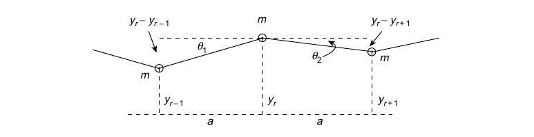
Fig 1. Displacements of three masses on a loaded string under tension T. Sourced from [1, p. 91].
The differential equation for each load is
\[ \ddot{y_r} = \frac{T}{ma}(y_{r-1}-2y_r+y_{r+1}) \]
Where \( m \) is the mass of the load which is the same and \( a \) is the horizontal distance from each load [1, p. 91].
I don’t know whether the \( m \) is actually \( m_r \) so that it doesn’t matter whether the loads’ masses are different or must it be uniform.
Say that we have \( n \) loads. If we fix the \( 0 \)th and \( n \)th load at \( y = 0 \) and \( \dot{y} = 0 \), we have a “string” that is tied at both ends. When \( n = 0 \) there are no moving loads, the same goes for \( n = 1 \) and \( n = 2 \). There is one moving load when \( n = 3 \) and two moving loads when \( n = 4 \). The number of moving loads is then defined as \( n - 2 \) when \( n \geq 3 \).
moving_loads = 20
n_loads = moving_loads+2

T = 1 # N
m = 1.5/n_loads # kg
a = 2/n_loads # m
We’ll use SciPy to solve our differential equation numerically. Before that, a bit of imports.
from scipy.integrate import solve_ivp
import matplotlib.pyplot as plt
import numpy as np
Our input to the function is \( [y_0, \dot{y_0}, y_1, \dot{y_1}, \cdots, y_n, \dot{y_n}] \), and that is why the output is \( [\dot{y_0}, \ddot{y_0}, \dot{y_1}, \ddot{y_1}, \cdots, \dot{y_n}, \ddot{y_n}] \).
Say that we have 4 loads, or in other words 2 moving loads. The differential equation will be
def diff(t, y):
    n_yp = n_loads*2 # there are n amounts of y dot and y double dots
    yp = np.zeros(n_yp) # place to store the differential equations (yp as in y prime)

    yp[0] = y[1]
    yp[1] = 0

    yp[2] = y[3]
    yp[3] = T/(m*a) * (y[0] - 2*y[2] + y[4])

    yp[4] = y[5]
    yp[5] = T/(m*a) * (y[2] - 2*y[4] + y[6])

    yp[6] = y[7]
    yp[7] = 0

    return yp
From that, we can see the generalized version using for loops is
def diff(t, y):
    n_ya = n_loads*2 # there are n amounts of y dot and y double dots
    ya = np.zeros(n_ya)

    for i in range(1, n_ya, 2):
        ya[i-1] = y[i]

    for i in range(3, n_ya-1, 2):
        ya[i] = T/(m*a) * (y[i-3] - 2*y[i-3+2] + y[i-3+4])

    ya[1] = 0
    ya[n_ya-1] = 0

    return np.array(ya)
Before solving the differential equation, we need initial values. Starting simple, we can just set the first moving load to some height or change its velocity to a non zero velocity to see what happens. After that we can set the initial values to one sine wave to see a standing wave, this is one of its normal modes.
# 1 Full Sine Wave
for i in range(2, points*2, 2):
    inits[i] = np.sin(np.pi/points*i)
Solving the differential equation using SciPy, we have
time = 5
inits = [0 for i in range(n_loads*2)]

# 1 Full Sine Wave
for i in range(2, points*2, 2):
    inits[i] = np.sin(np.pi/points*i)

# Remember, both the start and end loads are at y = 0
inits[0] = 0
inits[-2] = 0
sol = solve_ivp(
    diff,
    [0, time],
    inits,
    dense_output=True,
    rtol=1e-8
)

t = np.linspace(0, time, 100)
y = sol.sol(t)
To visualize what we have solved, I’ll use matplotlib’s animation functionality
from matplotlib import animation, rc
rc('animation', html='html5')

fig, ax = plt.subplots()
plt.close()

ax.set_xlim(0, a*(moving_loads+1))
ax.set_ylim(-1, 1)

ax.set_xlabel("x (m)")
ax.set_ylabel("y (m)")

loads = []

for i in range(n_loads):
    loads.append(ax.plot([], [], color="cornflowerblue", marker="o"))

text = ax.text(0.5, 0.5, 0, fontsize=12)
lines, = ax.plot([], [], color="orange")


def animate(i):
    text.set_text(f"{round(t[i], 2)} s")
    for j in range(n_loads):
        loads[j][0].set_data([a*j, y[j*2][i]])

    ass = [a*j for j in range(n_loads)]
    yss = [y[j*2][i] for j in range(n_loads)]

    lines.set_data([ass, yss])
    returns = loads + [lines]

    return tuple(returns)

anim = animation.FuncAnimation(fig, animate, frames=len(y[0]), blit=False, repeat=True, interval=1/24*1000)
anim
The end result looks something like this